Josh On Design

We've built a lot of stuff so far. In part one we built some tools and noise. In part two we created patterns with sine waves, then mixed them with noise. However, so far our images are essentially black and white, or occasionally hard coded to a particular color like red. Today we're going to lerp through some colors. Don't worry, I'll explain that this means in a minute.

All of our algorithms so far produce a number from 0 to 1 for each pixel. Color in computers is set with three components, Red, Green, and Blue. To color our output we can just set each component to the output value. This will produce a grayscale, since each component will always have the same value. To produce colors we could set the value in just one component, leaving the others as zero. That would give us shades of red, green, or blue; but not any combination. We could try to calculate some other colors by hand, but there's a better way to do this. Gradients

Gradients

A gradient (in computer science terms) is a single value that transitions between different values in a set. For example, if we have a gradient that goes from blue, to red, to orange, then we can calculate a value that transitions smoothly between them. The output color would go from blue, to redish purple, to red, to brown, to orange. To make this work we need a gradient function that accepts an input value and a set of colors. This function produces an output color that transition from the first to last colors in th set as the input goes from 0 to 1. Since our existing functions already produce values that go from 0 to 1 we can just plug them into this new function to colorize our output. The best part is that we can just switch gradients to completely change how the output looks.

The gradient functions can be tricky so let's build it up in pieces. The first thing we need is a function that goes between two values as the input goes from 0 to 1. This transition is called a Linear Interpolation because will be completely smooth and linear. It is commonly called a lerp for short.

function lerp(t,A,B) { return A + t*(B-A) }

We can use lerp to draw a black to white gradient across the image like this:

//lerp from 0 to 1. black to white
save(map(gen(100,100), (cur,px,py,ix,iy) => {
    const v = lerp(ix,0,1)
    return {r:v,g:v,b:v}
}), 'v3_1.png')

The lerp function works pretty well, but it only transitions between a starting and ending value. We want to go through a set of values, so let's create another function called lerps.

function lerps(t, values) {
    var band = Math.floor(t*(values.length-1));
    if(t === 1.0) band = (values.length-1)-1
    var band_size = 1/(values.length-1);
    var fract = (t-(band_size*band))/band_size;
    return lerp(fract,values[band],values[band+1]);
}

We can call lerps with an array of values. For example lerps(t,[10,30,5,8]) would start and 10, go up to 30, back down to 5, then up to 8; all as t goes from 0 to 1. Here's the code to go from black to white to black to white to black.

//lerp from 0 to 1 to 0 to 1 to 0
save(map(gen(100,100), (cur,px,py,ix,iy) => {
    const v = lerps(ix,[0,1,0,1,0])
    return {r:v,g:v,b:v}
}), 'v3_2.png')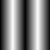

Of course we really want to lerp colors, not single values. We need just one more function.

function lerpRGBs(t, arr) {
    return {
        r: lerps(t, arr.map((C)=>C.r)),
        g: lerps(t, arr.map((C)=>C.g)),
        b: lerps(t, arr.map((C)=>C.b)),
    }
}

lerpRGBs can interpolate an array of colors like this:

const red   = { r:1, g:0, b:0 }
const green = { r:0, g:0, b:0 }
const black = { r:0, g:0, b:0 }
en(100,100), (cur,px,py,ix,iy) => {
    const c = lerpRGBs(ix,[red,green, black])
    return c
}), 'v3_3.png')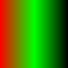

Sweet. Now let's see what happens when we use a gradient with our noise and sine functions from earlier.

//lerp two colors across some noise2D
save(map(gen(100,100), (cur,px,py,ix,iy) => {
    let theta = ix*2*pi
    theta += octave(ix,iy,8)*4
    const vx = sin(theta*4)
    let v = (1 + vx)/2 //map [-1,1] to [0-1]
    return lerpRGBs(v,[red,green])
}), 'v3_4.png')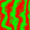

Woah! That looks cool. The code above calculates theta, then perturbs it by the noise, then uses that to make the sine wave. Finally the wave is colored with the gradient. The end result is the parts which would have been black in a pure noise function become the first color and the parts that would have been white become the second color.

Threholding

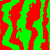
From this same base we can do some other funky things. How about a threshold. Instead of using a gradient just use the first or second color based on whether the value is below or above 0.5.

// use threshold on noise. red or green
save(map(gen(100,100), (cur,px,py,ix,iy) => {
    let theta = ix*2*pi 
    theta += octave(ix,iy,8)*4
    const vx = sin(theta*4)
    let v = (1 + vx)/2
    if(v < 0.5) return red
    return green
}), 'v3_5.png')

which gives us this

The boundary between red and green is a bit harsh. Let's divide the value into three sections. 0 to 0.4 will go to 0 (red), 0.6 to to 1.0 will go to 1 (green). The part in between 0.4 and 0.6 scaled back to 0-1, which will create a narrow gradient from red to green. The end result should look the same, but with a smoother boundary between the red and green sections.

save(map(gen(100,100), (cur,px,py,ix,iy) => {
    let theta = ix*2*pi
    theta += octave(ix,iy,8)*4
    const vx = sin(theta*4)
    let v = (1 + vx)/2
    if(v < 0.4) {
        v = 0
    } else if(v >= 0.6) {
        v = 1.0
    } else {
        v = (v-0.4)*5
    }
    return lerpRGBs(v,[red,green])
}), 'v3_6.png')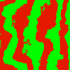

Or we could make the part less than 0.5 be red, and everything above be the normal noise field.

save(map(gen(100,100), (cur,px,py,ix,iy) => {
    let theta = ix*2*pi
    theta += octave(ix,iy,8)*4
    const vx = sin(theta*4)
    let v = (1 + vx)/2
    if(v < 0.5) {
        v = 0
    } else {
        v = (v-0.5)*2 // map [0.5,1.0] to [0.0,1.0]
    }
    return lerpRGBs(v,[red,green])
}), 'v3_7.png')

Now it looks sort of like a map where the flat portions are the water and the noisey green parts are the mountains. Of course the colors are wrong. Let's change the red part to a nice blue. I also adjusted some of the constants to make it feel more land-ish.

save(map(gen(100,100), (cur,px,py,ix,iy) => {
    let theta = ix*2*pi
    theta += octave(ix,iy,30)*5
    const vx = sin(theta*2)
    let v = (1 + vx)/2
    if(v < 0.5) {
        v = 0
    } else {
        v = (v-0.5)*2
    }
    return lerpRGBs(v,[seaBlue,brown])
}), 'v3_8.png')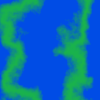

Putting it all together

As a final image, I created two functions that are mixed using thresholding. Anything below 0.5 will be red/green stripes. Anything above will be black/white stripes. The cool part is that it uses the noise function to determine the boundary between the two layers. I also changed the image size to be bigger. One of the great things about using headless code like this we can increase the size to whatever we want.

const white = {r:1, g:1, b:1}
save(map(gen(600,600), (cur,px,py,ix,iy) => {
    let theta1 = ix*2*pi // convert pixels to radians
    let theta2 = iy*2*pi // pixels to radians
    const vn = octave(ix,iy,30)
    let v1 = sin(theta1*3)
    let v2 = sin(theta2*4)
    v1 = (1 + v1)/2 //map [-1,1] to [0-1]
    v2 = (1 + v2)/2 //map [-1,1] to [0-1]
    if(vn < 0.5) {
        return lerpRGBs(v1,[red,green])
    } else {
        return lerpRGBs(v2,[black,white])
    }
}), 'v3_9.png')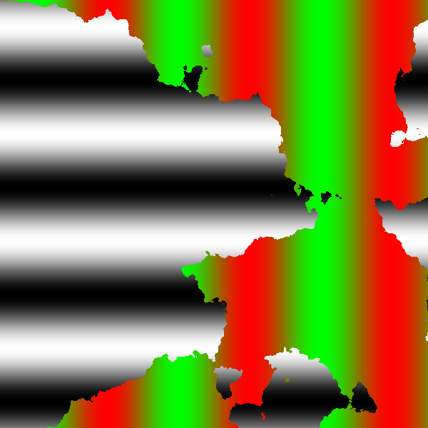

That's it for today. Let's see what tomorrow brings.